Neural network(1)---Logistic Regression
After a long time ,I decide to study Neural Network in a systematic way
Lead to
When I first talk about this topic, I want to use a Mathematical way to explain the algorithm---the Logistic Regression.fisrtly , I want to introduce this algorithm to you ,it is a tool to solve binary classification problem,firstly ,for a binary classification problem you may recall the function \(y=wx+b\),that is linear regression which is the simplest binary classification function ,if you have got the \(w,b\),and you input a \(x\),you will get a \(\hat y\), and if the actual value of \(y\) corresponding to \(x\) is bigger then \(\hat y\),or is smaller then \(\hat y\),you will use this way to get two two categories in much data
Overview of logistic regression
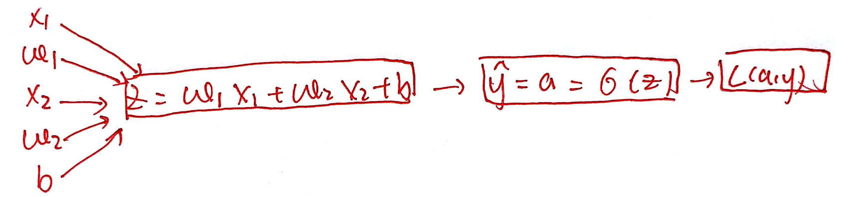
Today we will introduce a new algorithm to solve this problem: \[ \left\{\begin{array}{l} z=w^{\top} x+b \\ \hat{y}=a=\sigma(z) \\ L(a, y)=-(y \log (a)+(1-y) \log (1-a)) \end{array}\right. \]
you give the x and y ,you need give the initialization of \(w,b\) and program will help you to solve the \(\hat y\) and the loss function \(L(a,y)\) ,and the function \(\sigma(z)\) is \[ \sigma(z)=\frac{e^z}{e^z+1} \]
![]()
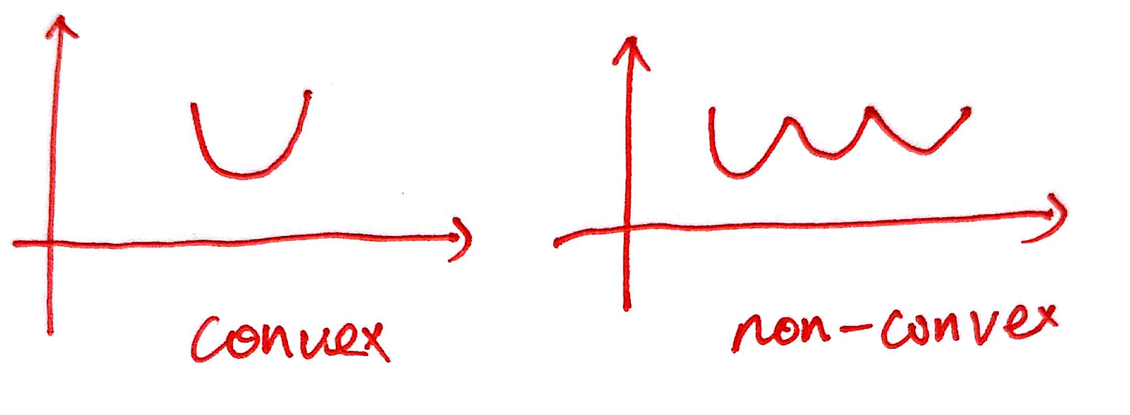
\(L\) is just like the \(\frac{1}{2}(y-\hat y)^2\),which represent how closer two points is ? if \(L\) is very small ,which represent the points is very closer. But why we don't choose \(\frac{1}{2}(y-\hat y)^2\),because if we choose this function ,the loss function is maybe not a convex function ,which exist many local minimize solve ,just like this picture :
when the loss function is non-convex ,the gradient can't work very well ,so we choose the another function as the loos function ,So why \(L(a,y)\) can be used to describe the distance ? just see two picture:
the two picture is the \(L(a,y)\),when I assume that y=0 and y=1 and the value of \(L\) is dependent on the value of a,
with different a,the \(L\) have different value ,when \(y=0\), only when \(a=0\),then the Probability also the \(L\) is equal to 1
1 represent True,0 represents False,so this is the reason why we choose this function to represents our "Loss function".
But unfortunately ,this value can't represent the overall performance on the model, so we need another function to reflect the accuracy of model ,so we introduce the \(J\) ,which is mean "Cost function" ,Its expression is : \[ J(w,b)=-\frac{1}{m}\sum_{i=1}^{m}(L(a^{(i)},y^{(i)})) \]
\[ dz=\frac{dl}{dz}=\frac{dl}{da}\cdot\frac{da}{dz}\\da=-\frac{y}{a}+\frac{1-y}{1-a} \]
so we can get : \[ \begin{equation}\begin{aligned}dz &=\frac{dl}{da}\cdot\frac{da}{dz}\\&=(-\frac{y}{a}+\frac{1-y}{1-a})\cdot \frac{e^z}{(e^z+1)^2}\\&=a(1-a)(-\frac{y}{a}+\frac{1-y}{1-a})\\&=a-y\end{aligned}\nonumber\end{equation} \] ok, we get the \(dz\),then we can get some other import information like this : \[ dw_1=\frac{\partial L}{\partial w_1}=x_1dz \qquad db =dz \] then we can use Gradient descent to update the \(w,b\): \[ \cases{w=w-\alpha w\\b=b-\alpha b} \] in this expression \(a^{(i)}=\hat y^{(i)}=\sigma(z^{(i)})=\sigma(w^Tx^{(i)+b})\).and we can calculate the derivative of \(J\) with respect to \(w\) and \(b\):
\[ \frac{\partial}{\partial w_i}J(w,b)=\frac{1}{m}\sum_{i=1}^{m}\frac{\partial}{\partial w_i}(L(a^{(i)},y^{(i)})) \] you can see : \[ \frac{\partial}{\partial w_i}(L(a^{(i)},y^{(i)}))=d w_{i}^{(i)}-\left(x^{(i)} \cdot y^{(i)}\right) \] so forward propagation just like this :
1 | J=0 dw_1=0 dw_2=0 db=0 |
Vectorization
whenever possible avoid explicit for loops
1 | For loop: |
if we use python-numpy:
1 | import numpy as np |
python-numpy's syntax is simpler, and calculation is more efficient,That is pretty good,deep learning need a lots of calculations ,so matrix syntax by numpy is recommended
Coding
Building this model neural network , let's do from the structure
- read the data and define the sigmoid function
- use data and sigmoid function to propagate the \(J\)
- use \(J\) to backpagate \(dw\) and \(db\)
- set number of iteration and learning rate to update the \(J\) (makes it smaller)
- predict the train data and the test data ,get the accuracy of model's prediction
- plot the \(J-n_{iteration}\) figure,see whether it is overfit or not ?
import lib and read data
1 | import numpy as np |
##data normalization
1 | train_set_x=train_set_x_flatten/255 |
define sigmoid
1 | def sigmoid(Z): #define sigmoid function |
1 | def initialize_with_zeros(dim): #Column vector |
propagation
1 | def Propagation(w,b,X,Y): |
define optimize
1 | def Propagation(w,b,X,Y): |
define predict
1 | def predict(w,b,X): |
model
1 | def model(X_train,Y_train,X_test,Y_test,num_iterations=2000,learning_rate=0.5,print_cost=False): |
1 | #test model |